Home-> Styles-> Conditional Formatting-> Icon Sets

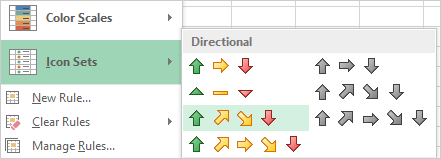
Use Icon Sets

Try It: Format with Icon Sets

Select Column H.

Go to Home -> Styles.

Go to Conditional Formatting.

Select Icon Sets: Arrows (Colored).

 

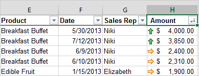
What Do You See? The Icon Sets use a three, four, or five-color scale to format the data.

In this example, there are four Directional arrows that represent the percentages of the total Amount in Column H:

100-75%

74-50%

49-25%
25-0%

 

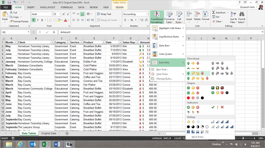
What Else Do You See? The Conditional Formatting menu also lets you create a New Rule or Manage the Rules.

 

Let's investigate where Excel puts the Rules and what tools are available in the Rules Manager.

Keep going...